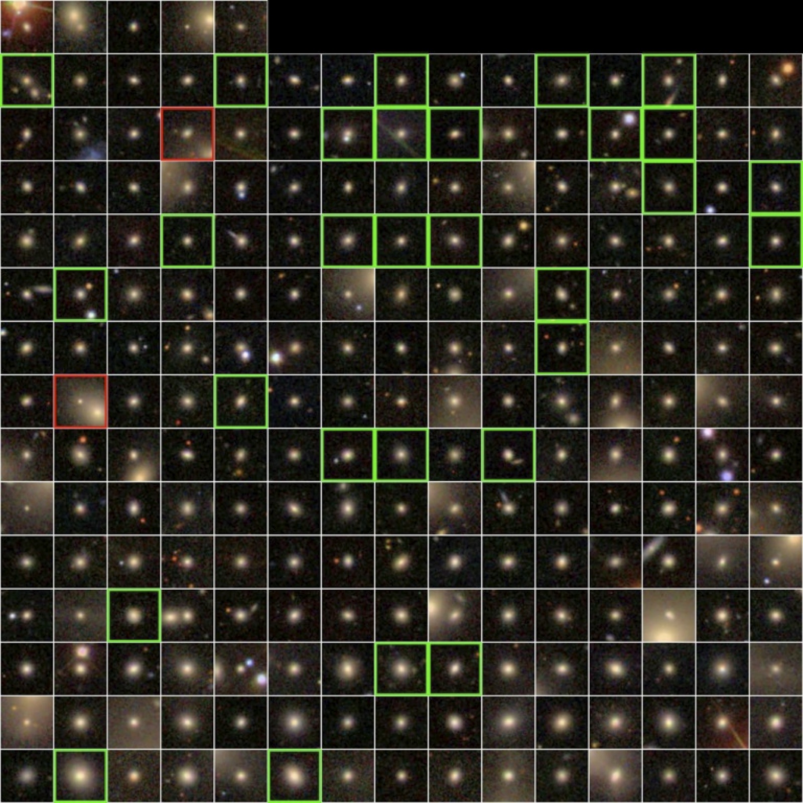
 A mosaics of compact elliptical galaxies thumbnails that can be selected from the RCSED data following this step-by-step guide.
Compact elliptical (cE) or Messier32-like galaxies are very dense and small stellar systems containing up-to several billion stars. They were considered extremely rare until recently: only a handful of them had been known until late 2000s when the first systematic cE search powered by the Virtual Observatory revealed two dozens of them residing in cores of nearby galaxy clusters observed with the Hubble Space Telescope. In 2012 Igor Chilingarian and Ivan Zolotukhin ran a tutorial at the ADASS meeting using a dataset which is now known as RCSED. They performed a search of cE which was independent of their environment, that is not only galaxy clusters, but also rich and sparse groups and even objects in isolation. They discovered about 200 new cEs in all types of environment, including 11 unique runaway galaxies ejected by large scale gravitational slingshots from their home clusters of galaxies into the emptiest regions of the Universe.
Here we propose a step-by-step guide to reproduce their study which resulted in a Science magazine publication. This guide exploits Virtual Observatory (VO, http://ivoa.net/) desktop applications such as TOPCAT, VOSpec and Aladin, and uses the RCSED catalog (a value-added Reference Catalog of Spectral Energy Distributions, http://rcsed.sai.msu.ru/) data.
Instruction
Before you begin
If you do not have the TOPCAT, VOSpec and Aladin applications installed on your workstation, you can either use Java WebStart (see below) or download standalone jar files using these links:
Launch applications on Linux (in terminal):
- TOPCAT:
java -jar topcat-lite.jar - VOSpec:
java -jar VOSpec_6.8.jar - Aladin:
java -jar Aladin.jar
- TOPCAT:
On Windows and Mac OS X they can be launched by double-clicking the downloaded jar files.
- Alternatively launch applications using Java WebStart, if your browser supports this method (many browsers do). Just click on these links (you may need to double click on the downloaded jnlp file and tell to open it with Java):
Step-by-step guide
Load the RCSED main table to TOPCAT by sending this SQL query to the RCSED data server:
File → Load table → DataSources → Table Access Protocol (TAP) Query → Keywords: rcsed → Find Services → select VOXAstro TAP → Use Service → Enter Query or directly copy-paste necessary URL TAP URL: http://rcsed-vo.sai.msu.ru/tap → Use Service → Enter Query:
SELECT
    objid, mjd, plate, fiberid, ra, dec,
    ssp_age, exp_tau, ssp_met, ssp_met_err, ssp_veldisp, ssp_veldisp, z,
    corrmag_nuv, corrmag_g, corrmag_r, corrmag_z, corrmag_k,
    kcorr_nuv, kcorr_g, kcorr_r, kcorr_z, kcorr_k, petror50_r
FROM
    specphot.rcsed
WHERE
    kcorr_k IS NOT NULL
Then click Run Query. This will create a table in the Table List namedTAP_1_specphot.rcsed.Note: in order to get a complete list of galaxies you need to change the Max Rows: "2000 (default)" to "20000000 (max)".
For a complete list of RCSED catalog tables and their columns with descriptions please see: http://rcsed.sai.msu.ru/docs/columns/. If this query result takes too long to load, you can just open RCSED main table FITS file in TOPCAT: File → Load Table → Location: https://zenodo.org/record/249750/files/rcsed.fits (219.3 MB)
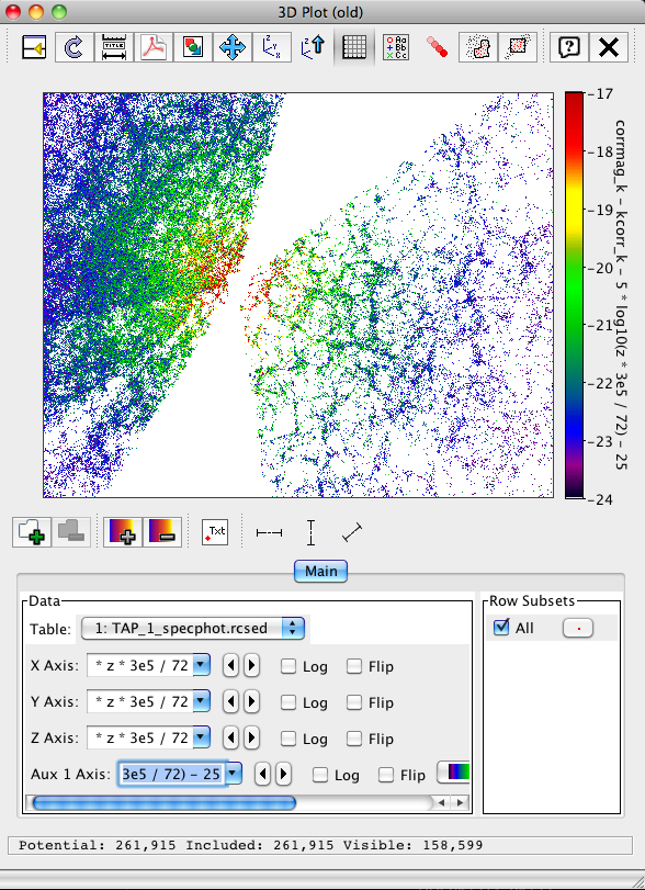
As a first exercise, we propose a visualisation of the Cosmic Web, the large-scale structure of the Universe, with galaxies colored according to their absolute K band magnitude which represents their stellar mass. For that purpose make a 3D plot (Graphics → 3D Plot (Old)) in TOPCAT with the following axes:
- X:
cos(ra / 57.3) * cos(dec / 57.3) * z * 3e5 / 72 - Y:
sin(ra / 57.3) * cos(dec / 57.3) * z * 3e5 / 72 - Z:
sin(dec / 57.3) * z * 3e5 / 72 - Click Add an auxiliary axis button:
corrmag_k - kcorr_k - 5 * log10(z * 3e5 / 72) - 25
Here 57.3 is a conversion from degrees to radians, 3e5 is speed of light in km/s, 72 is Hubble constant in km/s/Mpc (these approximate values serve well the illustration purpose). For better results set limits on color axis:
Plot → Configure Axes and Title → Color Range: from -24 to -17
and also do Rendering → Fog to turn it off. If you look on your plot from above and zoom, you should see inhomogeneous web-like distribution of galaxies like this:
Hint: it is actually much easier to do a 3D radial spherical plot (Graphics → Sphere Plot (Old) → click Plot points with radial...) and just add
z * 3e5 / 72as a radial coordinate to get essentially the same distribution.- X:
Add a new column,
gr_fit, using this expression (don't worry that it is so huge, just copy-paste it):Views → Column info → Columns → New Synthetic Column → Name:
gr_fitExpression:
0.0008569*pow((corrmag_z-kcorr_z-25-5 * log10(luminosityDistance(z,72.0,0.3,0.7))+21.6665),0) *
pow((corrmag_NUV-corrmag_r-kcorr_NUV+kcorr_r),0)  + 0.4145246 *
pow((corrmag_z-kcorr_z-25-5*log10(luminosityDistance(z,72.0,0.3,0.7)) + 21.6665),0) *
pow((corrmag_NUV-corrmag_r-kcorr_NUV+kcorr_r),1)  -0.3126628 *
pow((corrmag_z-kcorr_z-25-5*log10(luminosityDistance(z,72.0,0.3,0.7))+21.6665),0) *
pow((corrmag_NUV-corrmag_r-kcorr_NUV+kcorr_r),2)  +0.1915254 *
pow((corrmag_z-kcorr_z-25-5*log10(luminosityDistance(z,72.0,0.3,0.7))+21.6665),0) *
pow((corrmag_NUV-corrmag_r-kcorr_NUV+kcorr_r),3)  -0.0604829 *
pow((corrmag_z-kcorr_z-25-5*log10(luminosityDistance(z,72.0,0.3,0.7))+21.6665),0) *
pow((corrmag_NUV-corrmag_r-kcorr_NUV+kcorr_r),4)  +0.0100710 *
pow((corrmag_z-kcorr_z-25-5*log10(luminosityDistance(z,72.0,0.3,0.7))+21.6665),0) *
pow((corrmag_NUV-corrmag_r-kcorr_NUV+kcorr_r),5)  -0.0008631 *
pow((corrmag_z-kcorr_z-25-5*log10(luminosityDistance(z,72.0,0.3,0.7))+21.6665),0) *
pow((corrmag_NUV-corrmag_r-kcorr_NUV+kcorr_r),6)  +0.0000304 *
pow((corrmag_z-kcorr_z-25-5*log10(luminosityDistance(z,72.0,0.3,0.7))+21.6665),0) *
pow((corrmag_NUV-corrmag_r-kcorr_NUV+kcorr_r),7)  +0.1037934 *
pow((corrmag_z-kcorr_z-25-5*log10(luminosityDistance(z,72.0,0.3,0.7))+21.6665),1) *
pow((corrmag_NUV-corrmag_r-kcorr_NUV+kcorr_r),0)  -0.2982120 *
pow((corrmag_z-kcorr_z-25-5*log10(luminosityDistance(z,72.0,0.3,0.7))+21.6665),1) *
pow((corrmag_NUV-corrmag_r-kcorr_NUV+kcorr_r),1)  +0.2527798 *
pow((corrmag_z-kcorr_z-25-5*log10(luminosityDistance(z,72.0,0.3,0.7))+21.6665),1) *
pow((corrmag_NUV-corrmag_r-kcorr_NUV+kcorr_r),2)  -0.1029656 *
pow((corrmag_z-kcorr_z-25-5*log10(luminosityDistance(z,72.0,0.3,0.7))+21.6665),1) *
pow((corrmag_NUV-corrmag_r-kcorr_NUV+kcorr_r),3)  +0.0219900 *
pow((corrmag_z-kcorr_z-25-5*log10(luminosityDistance(z,72.0,0.3,0.7))+21.6665),1) *
pow((corrmag_NUV-corrmag_r-kcorr_NUV+kcorr_r),4)  -0.0023795 *
pow((corrmag_z-kcorr_z-25-5*log10(luminosityDistance(z,72.0,0.3,0.7))+21.6665),1) *
pow((corrmag_NUV-corrmag_r-kcorr_NUV+kcorr_r),5)  +0.0001031 *
pow((corrmag_z-kcorr_z-25-5*log10(luminosityDistance(z,72.0,0.3,0.7))+21.6665),1) *
pow((corrmag_NUV-corrmag_r-kcorr_NUV+kcorr_r),6)  -0.0146987 *
pow((corrmag_z-kcorr_z-25-5*log10(luminosityDistance(z,72.0,0.3,0.7))+21.6665),2) *
pow((corrmag_NUV-corrmag_r-kcorr_NUV+kcorr_r),0)  +0.0487196 *
pow((corrmag_z-kcorr_z-25-5*log10(luminosityDistance(z,72.0,0.3,0.7))+21.6665),2) *
pow((corrmag_NUV-corrmag_r-kcorr_NUV+kcorr_r),1)  -0.0351197 *
pow((corrmag_z-kcorr_z-25-5*log10(luminosityDistance(z,72.0,0.3,0.7))+21.6665),2) *
pow((corrmag_NUV-corrmag_r-kcorr_NUV+kcorr_r),2)  +0.0100174 *
pow((corrmag_z-kcorr_z-25-5*log10(luminosityDistance(z,72.0,0.3,0.7))+21.6665),2) *
pow((corrmag_NUV-corrmag_r-kcorr_NUV+kcorr_r),3)  -0.0012482 *
pow((corrmag_z-kcorr_z-25-5*log10(luminosityDistance(z,72.0,0.3,0.7))+21.6665),2) *
pow((corrmag_NUV-corrmag_r-kcorr_NUV+kcorr_r),4)  +0.0000568 *
pow((corrmag_z-kcorr_z-25-5*log10(luminosityDistance(z,72.0,0.3,0.7))+21.6665),2) *
pow((corrmag_NUV-corrmag_r-kcorr_NUV+kcorr_r),5)  +0.0003963 *
pow((corrmag_z-kcorr_z-25-5*log10(luminosityDistance(z,72.0,0.3,0.7))+21.6665),3) *
pow((corrmag_NUV-corrmag_r-kcorr_NUV+kcorr_r),0)  -0.0029259 *
pow((corrmag_z-kcorr_z-25-5*log10(luminosityDistance(z,72.0,0.3,0.7))+21.6665),3) *
pow((corrmag_NUV-corrmag_r-kcorr_NUV+kcorr_r),1)  +0.0021275 *
pow((corrmag_z-kcorr_z-25-5*log10(luminosityDistance(z,72.0,0.3,0.7))+21.6665),3) *
pow((corrmag_NUV-corrmag_r-kcorr_NUV+kcorr_r),2)  -0.0004860 *
pow((corrmag_z-kcorr_z-25-5*log10(luminosityDistance(z,72.0,0.3,0.7))+21.6665),3) *
pow((corrmag_NUV-corrmag_r-kcorr_NUV+kcorr_r),3)  +0.0000349 *
pow((corrmag_z-kcorr_z-25-5*log10(luminosityDistance(z,72.0,0.3,0.7))+21.6665),3) *
pow((corrmag_NUV-corrmag_r-kcorr_NUV+kcorr_r),4)
This polynomial is the universal optical–ultraviolet color–color–magnitude relation (surface) for normal galaxies (see http://rcsed.sai.msu.ru/article/universal-photometric-relation-for-galaxies/ and http://rcsed.sai.msu.ru/galaxy-colors/). The complete description of the used analytic expression is provided in this paper: http://adsabs.harvard.edu/abs/2010MNRAS.405.1409C.
Create a 3D plot using following axes, which represent the magnitude–color–color (Mz, NUV-r, g-r) parameter space:
- X:
corrmag_z - kcorr_z - 25 - 5 * log10(z * 3e5 / 72.0) - Y:
corrmag_NUV - corrmag_r - kcorr_NUV + kcorr_r - Z:
corrmag_g - corrmag_r - kcorr_g + kcorr_r
After inserting these expressions for the coordinates of the axes, please set the following axes limits for better plot appearance:
- X Range: from -25 to -16
- Y Range: from 0 to 7
- Z Range: from 0 to 1
- X:
Add a new 3D plot to the previous one (click Add new dataset button in the plot window) using the
gr_fitcolumn as Z axis keeping same X and Y axes (new Z Range: from 0 to 1). This plot represents the universal optical–ultraviolet color–color–magnitude relation (surface) for normal galaxies (see http://adsabs.harvard.edu/abs/2012MNRAS.419.1727C for the original paper and coefficients of the surface that we have entered when creatinggr_fitcolumn at step #3):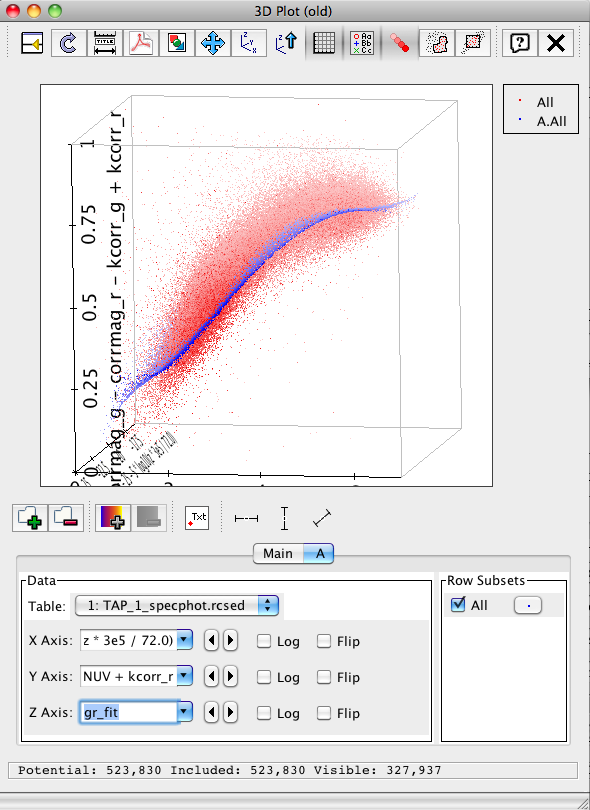
Select continuous region of candidate cE (compact elliptical galaxies) outliers which reside above the fitted surface
gr_fitat low luminosity part. You can draw the selection by hand (menu Subsets → Draw Subset Region) but for more formal criterion we suggest you to make the following filter in TOPCAT:Views → Row Subsets → Subsets → New subset → Name: cE
Expression:
(corrmag_NUV - corrmag_r - kcorr_NUV + kcorr_r) > 4.0 &&
(corrmag_g - kcorr_g - 25 - 5 * log10(luminosityDistance(z, 72.0, 0.3, 0.7))) > -18.7 &&
(petror50_r < 2.0 || petror50_r / 206.265 * luminosityDistance(z, 72.0, 0.3, 0.7) < 0.7) &&
(corrmag_g - corrmag_r - kcorr_g + kcorr_r - gr_fit) > 0.03 && ssp_age > 4000.0 &&
ssp_veldisp > 60.0
We also found it useful to change the last condition to:
(ssp_veldisp > 60.0 || exp_veldisp > 60.0).To see the images of selected cE candidates in the SDSS data:
In TOPCAT in the main window: choose Row Subset: cE and also Activation Action → Transmit Coordinates. To display all cE galaxies in the SDSS field do Interop → Broadcast table, they then pop up in Aladin window.
In Aladin: File → All sky → Image → Optical → SDSS colored to load all sky SDSS image and zoom to the desired level of details. Once you click on a row in TOPCAT, Aladin will re-point to an object's coordinates in SDSS imagery and you will be able to see its image.
Verify cE candidates by inspecting their spectra – cE galaxies do not possess any emission lines so by looking at spectra of candidates one can discard false matches. There are two options to do this:
- In main TOPCAT window do: Activation Action → View URL as Image → Image Location column:
"http://rcsed.sai.msu.ru/plot_spectrum_sed_stamp/?plate=" + toString(plate) + "&mjd=" + toString(mjd) + "&fiberid=" + toString(fiberid) + "&smooth=5"→ Image Format: PNG → OK and then click on rows of a table or points in any diagram to see an overview of a spectrum and a thumbnail of a galaxy. Change URL to"http://rcsed.sai.msu.ru/plot_spectrum_emis/?plate=" + toString(plate) + "&mjd=" + toString(mjd) + "&fiberid=" + toString(fiberid) + "&smooth=5"to see spectrum details upon activating any table row. - Download real spectra using RCSED SSAP service (endpoint URL is http://rcsed-vo.sai.msu.ru/specphot/ssap.q/ssa/ssap.xml). To do this first make a query to the spectral service by coordinates: VO → Multiple SSA → Keywords: rcsed → Find Services → select RCSED_SSAP → Input table: TAP_1_specphot.rcsed → Search Radius column: 3 → Go in TOPCAT to download spectral metadata for all candidates at once. This will create table
ssas(1)in your TOPCAT window. You can explore these spectra further in VOSpec by choosing in the main window of TOPCAT whenssas(1)is selected in the list of tables: Activation Action → View URL as Spectrum → Spectrum Location column: accref → Spectrum Viewer: VOSpec. VOSpec has to be launched beforehand. Then click on any row ofssas(1)table and see galaxy spectrum loaded in VOSpec.
- In main TOPCAT window do: Activation Action → View URL as Image → Image Location column:
At this step you have a list of compact galaxies with colors and luminosities similar to known cE galaxes which do not exhibit emission lines just like real cE galaxies. Hence you have just built a sample of bona-fide cE candidates.
Bonus part
Check the HST archive at CADC for better imaging data using ObsTAP access and
caom.pyscript (contact us through feedback to get a copy).Load the value-added catalog of Groups and clusters of galaxies in the SDSS DR8 by Tempel et al. (2012) either from VizieR or from the local disk and cross-match it with RCSED catalog using the 3 arcsec "sky" match. You may want to restart TOPCAT before doing cross-match of half a million rows tables using the following command in the terminal to give it more memory:
java -Xmx400M -jar topcat-full.jar. Filter resulting table by meaningful absolute z magnitude (corrmag_z - kcorr_z - 25 - 5 * log10(luminosityDistance(z_1, 72.0, 0.3, 0.7))) and make it a default subset.Create 3D plot using following axes which represent evolution of luminosity-metallicity relation depending on galaxy group size:
- X:
ssp_met - Y:
Nrich(and tick flip axis for convenience) - Z:
corrmag_z - kcorr_z - 25 - 5 * log10(luminosityDistance(z_1, 72.0, 0.3, 0.7))
When you explore this figure, it becomes evident, that luminosity-metallicity relation gets much wider for the field galaxies and it only exists essentially in groups.
- X: